library(httr2)Warning: package 'httr2' was built under R version 4.4.3library(jsonlite)
library(dplyr)
library(ggplot2)
library(DT)Warning: package 'DT' was built under R version 4.4.3Querying and visualizing deforestation data using PRODES as source
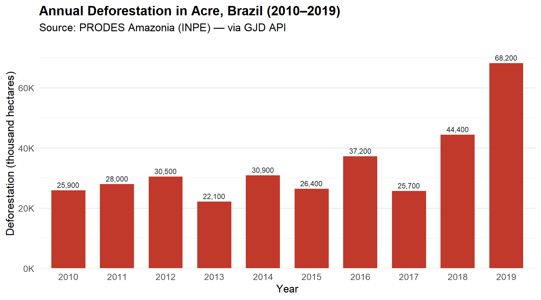
In this use case we shift our focus from forest cover to deforestation. We will query annual deforestation data for Acre, Brazil from 2010 to 2019, using data from PRODES — the official Brazilian deforestation monitoring system operated by INPE.
This example also demonstrates an important aspect of the GJD API: filtering by data source, since multiple sources may report on the same topic for the same jurisdiction.
Make sure you have completed the Get Started and API Authentication sections before running this notebook.
library(httr2)Warning: package 'httr2' was built under R version 4.4.3library(jsonlite)
library(dplyr)
library(ggplot2)
library(DT)Warning: package 'DT' was built under R version 4.4.3For this use case:
| Parameter | Value | Meaning |
|---|---|---|
ID_Topic |
11 |
Deforestation |
ID_Countries |
["BR"] |
Brazil |
ID_Jurisdictions |
["BR-AC"] |
Acre |
ID_years |
["2010", ..., "2019"] |
Years 2010–2019 |
ID_sources |
[12] |
PRODES Amazonia, Brazil |
The GJD API may return data from multiple sources for the same topic and jurisdiction. For example, deforestation in Acre is reported by PRODES, Hansen/UMD/Google, and MapBiomas — each using different methodologies and yielding different values. By specifying ID_sources=[12], we ensure we only get PRODES data for consistency.
base_url <- "https://api.greenjurisdictions.org/api/v1/dataPlaces/false/true/false"

years <- paste0('"', 2010:2019, '"', collapse = ",")

query_params <- list(
  ID_Topic         = 11,
  ID_Countries     = '["BR"]',
  ID_Jurisdictions = '["BR-AC"]',
  ID_Municipalities = '[]',
  ID_years         = paste0("[", years, "]"),
  ID_sources       = '[12]'
)

response <- request(base_url) |>
  req_url_query(!!!query_params) |>
  req_headers(
    "X-API-TOKEN"  = Sys.getenv("GJD_API_KEY"),
    "Accept"       = "application/json",
    "Content-Type" = "application/json"
  ) |>
  req_perform()

cat("HTTP status:", resp_status(response), "\n")
HTTP status: 200 body <- resp_body_json(response, simplifyVector = TRUE)
cat("Message:", body$message, "\n")Message: Resources retrieved successfully. cat("Total records:", body$data$total_data, "\n")Total records: 10 df <- body$data$data |>
as_tibble() |>
mutate(
value = as.numeric(value),
year = as.integer(year)
) |>
select(year, jurisdiction, value, unit, source) |>
arrange(year)
glimpse(df)Rows: 10
Columns: 5
$ year <int> 2010, 2011, 2012, 2013, 2014, 2015, 2016, 2017, 2018, 2019
$ jurisdiction <chr> "Acre", "Acre", "Acre", "Acre", "Acre", "Acre", "Acre", "…
$ value <dbl> 25900, 28000, 30500, 22100, 30900, 26400, 37200, 25700, 4…
$ unit <chr> "hectares", "hectares", "hectares", "hectares", "hectares…
$ source <chr> "PRODES Amazonia, Brazil", "PRODES Amazonia, Brazil", "PR…df |>
datatable(
caption = "Annual deforestation in Acre, Brazil (2010–2019) — PRODES",
colnames = c("Year", "Jurisdiction", "Deforestation", "Unit", "Source"),
options = list(
pageLength = 10,
dom = "tip"
),
rownames = FALSE
) |>
formatRound("value", digits = 0, mark = ",")ggplot(df, aes(x = factor(year), y = value / 1e3)) +
geom_col(fill = "#c0392b", width = 0.7) +
geom_text(
aes(label = scales::comma(value, accuracy = 1)),
vjust = -0.5, size = 3, color = "#17252a"
) +
scale_y_continuous(
labels = scales::comma_format(suffix = "K"),
expand = expansion(mult = c(0, 0.12))
) +
labs(
title = "Annual Deforestation in Acre, Brazil (2010–2019)",
subtitle = "Source: PRODES Amazonia (INPE) — via GJD API",
x = "Year",
y = "Deforestation (thousand hectares)"
) +
theme_minimal(base_size = 13) +
theme(
plot.title = element_text(face = "bold"),
panel.grid.major.x = element_blank()
)
To illustrate why source filtering matters, let’s make the same request without the ID_sources filter and see what we get.
query_all_sources <- list(
  ID_Topic         = 11,
  ID_Countries     = '["BR"]',
  ID_Jurisdictions = '["BR-AC"]',
  ID_Municipalities = '[]',
  ID_years         = paste0("[", years, "]")
)

response_all <- request(base_url) |>
  req_url_query(!!!query_all_sources) |>
  req_headers(
    "X-API-TOKEN"  = Sys.getenv("GJD_API_KEY"),
    "Accept"       = "application/json",
    "Content-Type" = "application/json"
  ) |>
  req_perform()

body_all <- resp_body_json(response_all, simplifyVector = TRUE)

df_all <- body_all$data$data |>
  as_tibble() |>
  mutate(
    value = as.numeric(value),
    year  = as.integer(year)
  ) |>
  select(year, jurisdiction, value, unit, source) |>
  arrange(year, source)

cat("Records with all sources:", nrow(df_all), "\n")
Records with all sources: 30 cat("Sources found:", paste(unique(df_all$source), collapse = ", "), "\n")Sources found: Hansen et al./UMD/Google/USGS/NASA, post-processing by EII, MapBiomas - Brasil, PRODES Amazonia, Brazil Now let’s visualize how the three sources compare:
ggplot(df_all, aes(x = factor(year), y = value / 1e3, fill = source)) +
  geom_col(position = "dodge", width = 0.7) +
  scale_fill_manual(values = c(
    "PRODES Amazonia, Brazil" = "#c0392b",
    "Hansen et al./UMD/Google/USGS/NASA, post-processing by EII" = "#2980b9",
    "MapBiomas - Brasil" = "#27ae60"
  )) +
  scale_y_continuous(
    labels = scales::comma_format(suffix = "K"),
    expand = expansion(mult = c(0, 0.08))
  ) +
  labs(
    title    = "Deforestation in Acre: Comparing Data Sources (2010–2019)",
    subtitle = "Three sources report different values for the same jurisdiction and topic",
    x        = "Year",
    y        = "Deforestation (thousand hectares)",
    fill     = "Data Source"
  ) +
  theme_minimal(base_size = 12) +
  theme(
    plot.title       = element_text(face = "bold"),
    panel.grid.major.x = element_blank(),
    legend.position  = "bottom",
    legend.direction = "vertical"
  )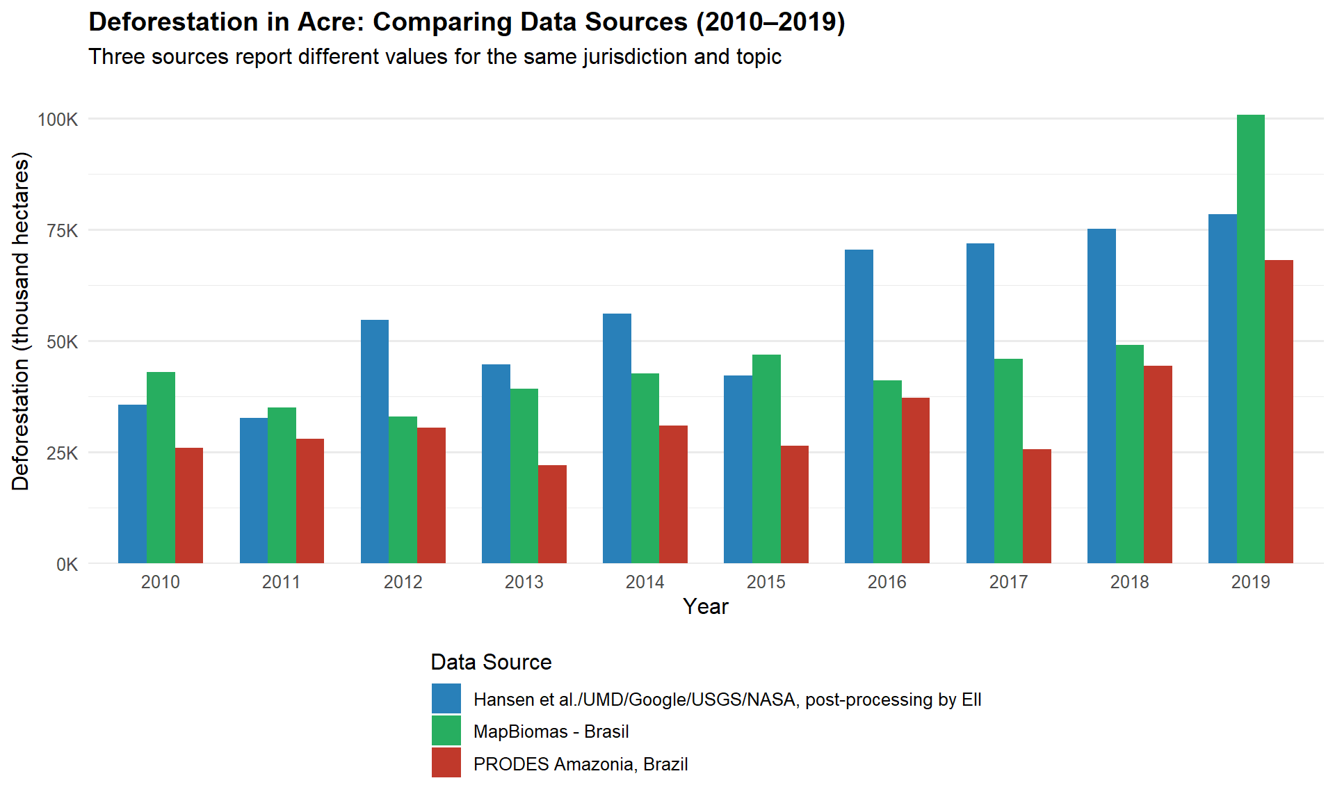
Different data sources use different methodologies (satellite imagery resolution, classification algorithms, reference periods). Always be explicit about which source you are using in your analysis and document your choice.
In this use case we learned how to:
ggplot2.