install.packages(c("sf", "geojsonsf"))UC03: Spatial Deforestation in Caquetá & Putumayo (Municipalities)
Fetching municipal-level GeoJSON data from the GJD API and rendering maps with ggplot2
Objective
In this use case we fetch deforestation data with municipality-level geometry for all 29 municipalities of Caquetá and Putumayo (Colombia) from the GJD API. The API returns paginated GeoJSON (10 features per page), so we collect all pages and assemble a single spatial dataset. We render two static maps using ggplot2 + sf:
- Basic map — Display all municipalities with labeled boundaries.
- Choropleth map — Color each municipality by its deforestation value.
Prerequisites
Make sure you have completed the Get Started and API Authentication sections. You will also need the sf and geojsonsf packages:
Step 1: Load Libraries
readRenviron("../.Renviron")
library(httr2)
Warning: package 'httr2' was built under R version 4.4.3library(jsonlite)
library(dplyr)
library(ggplot2)
library(sf)Warning: package 'sf' was built under R version 4.4.3library(geojsonsf)Warning: package 'geojsonsf' was built under R version 4.4.3Step 2: Build the API Request
The GJD API can return GeoJSON by adding geojson=true to the query. We request deforestation data (topic_id 11) for all municipalities of Caquetá (16) and Putumayo (13) for the year 2019, using IDEAM as the source.
Note: For GeoJSON requests, the API uses the parameter
topic_idinstead ofID_Topic. The API returns paginated results (10 features per page), so we loop through all pages.
| Parameter | Value | Meaning |
|---|---|---|
topic_id |
11 |
Deforestation |
ID_Countries |
["CO"] |
Colombia |
ID_Jurisdictions |
["CO-CAQ","CO-PUT"] |
Caquetá and Putumayo |
ID_Municipalities |
[29 codes] |
All municipalities |
ID_years |
["2019"] |
Year 2019 |
ID_sources |
[14] |
IDEAM, Colombia |
geojson |
true |
Include geometry |
base_url <- "https://api.greenjurisdictions.org/api/v1/dataPlaces/false/false/false"

municipalities <- c(
  "CO-CAQ-18029", "CO-CAQ-18094", "CO-CAQ-18150", "CO-CAQ-18205",
  "CO-CAQ-18247", "CO-CAQ-18256", "CO-CAQ-18001", "CO-CAQ-18460",
  "CO-CAQ-18410", "CO-CAQ-18479", "CO-CAQ-18592", "CO-CAQ-18610",
  "CO-CAQ-18753", "CO-CAQ-18756", "CO-CAQ-18785", "CO-CAQ-18860",
  "CO-PUT-86219", "CO-PUT-86001", "CO-PUT-86320", "CO-PUT-86568",
  "CO-PUT-86569", "CO-PUT-86571", "CO-PUT-86573", "CO-PUT-86755",
  "CO-PUT-86757", "CO-PUT-86760", "CO-PUT-86749", "CO-PUT-86865",
  "CO-PUT-86885"
)

query_params <- list(
  topic_id          = 11,
  ID_Countries      = '["CO"]',
  ID_Jurisdictions  = '["CO-CAQ","CO-PUT"]',
  ID_Municipalities = toJSON(municipalities),
  ID_years          = '["2019"]',
  ID_sources        = '[14]',
  ID_Classes        = '[]',
  api               = 'true',
  lang              = 'en',
  type              = 'api',
  geojson           = 'true'
)
Step 3: Fetch All Pages and Assemble GeoJSON
all_features <- list()
page <- 1

repeat {
  params <- c(query_params, list(page = page))

  response <- request(base_url) |>
    req_url_query(!!!params) |>
    req_headers(
      "X-API-TOKEN"  = Sys.getenv("GJD_API_KEY"),
      "Accept"       = "application/json",
      "Content-Type" = "application/json"
    ) |>
    req_perform()

  body <- resp_body_json(response)
  pag  <- body$data$data
  feats <- pag$data$features

  all_features <- c(all_features, feats)
  cat(sprintf("Page %d: %d features (total: %d)\n", page, length(feats), pag$total))

  if (page >= pag$last_page) break
  page <- page + 1
}
Page 1: 10 features (total: 29)
Page 2: 10 features (total: 29)
Page 3: 9 features (total: 29)cat(sprintf("\nTotal features collected: %d\n", length(all_features)))
Total features collected: 29Step 4: Convert to Spatial Data
We build a GeoJSON FeatureCollection from the collected features and convert it to an sf object:
as_list_recursive <- function(x) {
  if (is.list(x)) return(lapply(x, as_list_recursive))
  if (!is.null(names(x))) return(as.list(x))
  x
}

geojson_fc <- as_list_recursive(
  list(type = "FeatureCollection", features = all_features)
)
geojson_str <- toJSON(geojson_fc, auto_unbox = TRUE)

sf_data <- geojson_sf(geojson_str)

sf_data$value <- as.numeric(sf_data$value)
sf_data$jurisdiction <- ifelse(
  grepl("^CO-CAQ", sf_data$place_code), "Caquetá", "Putumayo"
)

cat("Municipalities loaded:", nrow(sf_data), "\n")
Municipalities loaded: 29 glimpse(sf_data)Rows: 29
Columns: 8
$ unit_id <dbl> 1, 1, 1, 1, 1, 1, 1, 1, 1, 1, 1, 1, 1, 1, 1, 1, 1, 1, 1, …
$ year <dbl> 2019, 2019, 2019, 2019, 2019, 2019, 2019, 2019, 2019, 201…
$ place_code <chr> "CO-CAQ-18592", "CO-PUT-86573", "CO-CAQ-18001", "CO-PUT-8…
$ value <dbl> 449.122, 2428.561, 159.551, 0.000, 80.766, 4094.180, 3418…
$ variable_id <dbl> 1100000, 1100000, 1100000, 1100000, 1100000, 1100000, 110…
$ source_id <dbl> 14, 14, 14, 14, 14, 14, 14, 14, 14, 14, 14, 14, 14, 14, 1…
$ geometry <MULTIPOLYGON [°]> MULTIPOLYGON (((-75.0554 2...., MULTIPOLYGON…
$ jurisdiction <chr> "Caquetá", "Putumayo", "Caquetá", "Putumayo", "Caquetá", …Step 5: Basic Map
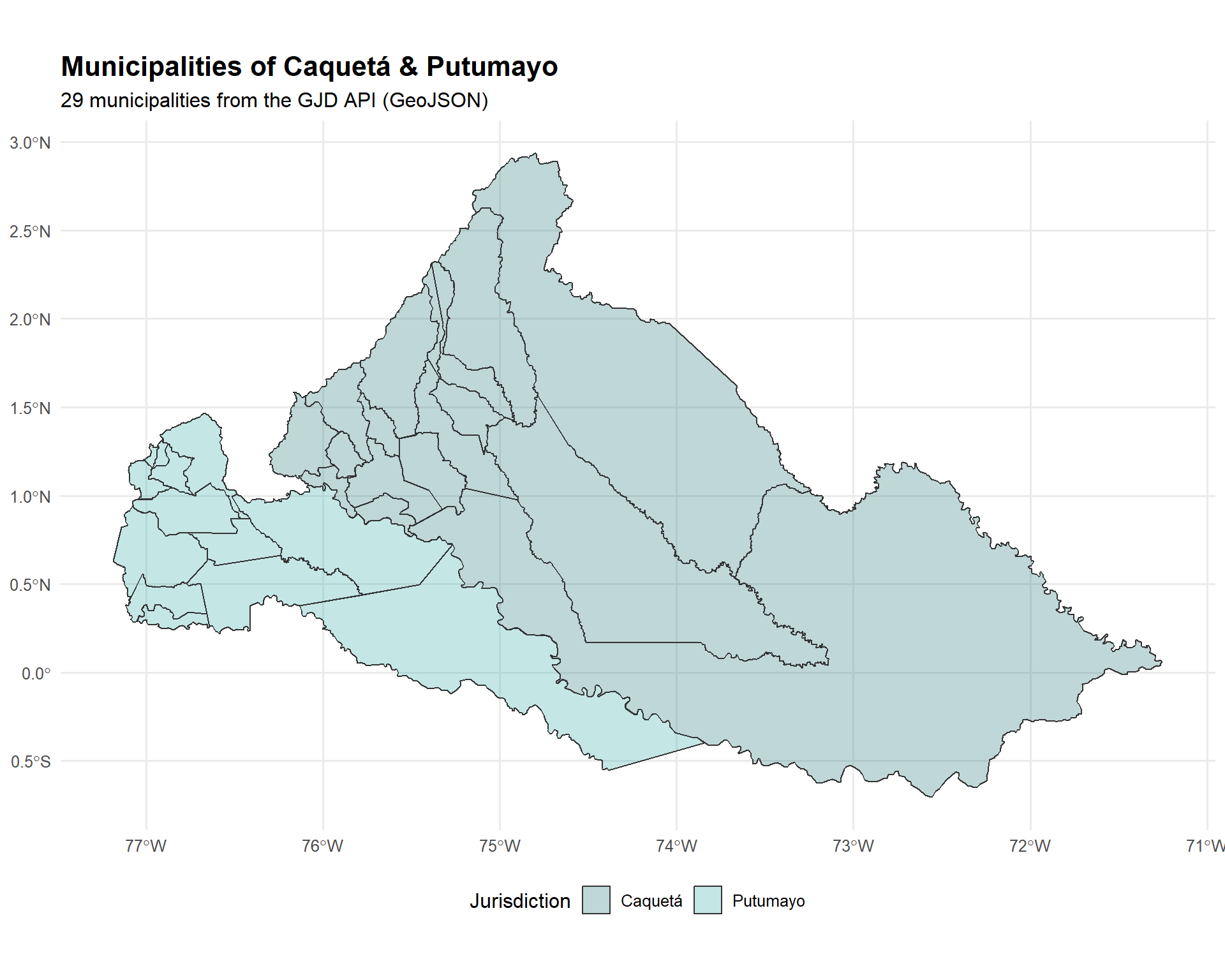
Display all 29 municipalities with their boundaries, colored by jurisdiction.
centroids <- st_centroid(sf_data)Warning: st_centroid assumes attributes are constant over geometriescoords <- st_coordinates(centroids)
sf_data$label_x <- coords[, 1]
sf_data$label_y <- coords[, 2]
ggplot(sf_data) +
geom_sf(aes(fill = jurisdiction), color = "#333", linewidth = 0.4, alpha = 0.3) +
scale_fill_manual(values = c("Caquetá" = "#2b7a78", "Putumayo" = "#3aafa9")) +
labs(
title = "Municipalities of Caquetá & Putumayo",
subtitle = "29 municipalities from the GJD API (GeoJSON)",
fill = "Jurisdiction"
) +
theme_minimal(base_size = 12) +
theme(
plot.title = element_text(face = "bold", size = 16),
legend.position = "bottom"
)
Step 6: Choropleth Map — Color by Deforestation
Each municipality is colored according to its deforestation value for 2019. Labels show the municipality code.
ggplot(sf_data) +
  geom_sf(aes(fill = value), color = "#333", linewidth = 0.4) +
  scale_fill_gradient(
    low  = "#fee5d9",
    high = "#a50f15",
    name = "Deforestation\n(hectares)",
    labels = scales::comma
  ) +
  geom_sf_text(
    aes(label = gsub("CO-(CAQ|PUT)-", "", place_code)),
    size = 2.5, color = "#333", fontface = "bold",
    check_overlap = TRUE
  ) +
  labs(
    title = "Deforestation by Municipality (2019)",
    subtitle = "Caquetá & Putumayo — Source: IDEAM via GJD API",
    caption = "Municipality codes shown as labels"
  ) +
  theme_minimal(base_size = 12) +
  theme(
    plot.title    = element_text(face = "bold", size = 16),
    plot.subtitle = element_text(color = "gray40"),
    plot.caption  = element_text(color = "gray60", size = 9),
    legend.position = "right"
  )
Warning in st_point_on_surface.sfc(sf::st_zm(x)): st_point_on_surface may not
give correct results for longitude/latitude data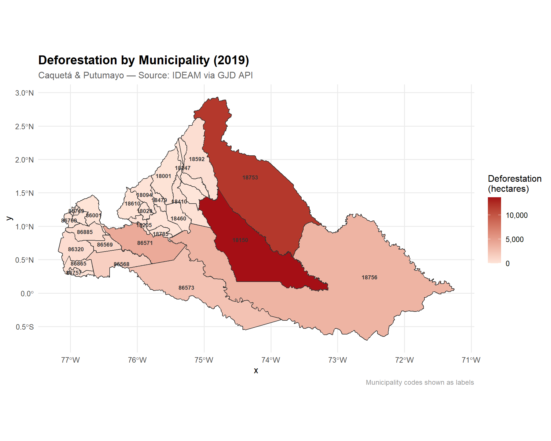
The map clearly highlights that municipalities like 18150 (San Vicente del Caguán) and 18753 (San José del Fragua) in Caquetá have the highest deforestation values in 2019.
Step 7: Top 10 Municipalities Table
sf_data |>
  st_drop_geometry() |>
  select(place_code, jurisdiction, value) |>
  arrange(desc(value)) |>
  head(10) |>
  mutate(value = format(round(value, 2), big.mark = ",")) |>
  knitr::kable(
    col.names = c("Municipality Code", "Jurisdiction", "Deforestation (ha)"),
    align = c("l", "l", "r"),
    caption = "Top 10 municipalities by deforestation (2019)"
)| Municipality Code | Jurisdiction | Deforestation (ha) |
|---|---|---|
| CO-CAQ-18150 | Caquetá | 13,672.27 |
| CO-CAQ-18753 | Caquetá | 11,884.27 |
| CO-PUT-86571 | Putumayo | 4,094.18 |
| CO-CAQ-18756 | Caquetá | 3,418.80 |
| CO-PUT-86573 | Putumayo | 2,428.56 |
| CO-PUT-86568 | Putumayo | 1,540.32 |
| CO-PUT-86569 | Putumayo | 994.11 |
| CO-PUT-86320 | Putumayo | 592.63 |
| CO-PUT-86885 | Putumayo | 561.40 |
| CO-CAQ-18592 | Caquetá | 449.12 |
Summary
In this use case we learned how to:
- Request municipal-level GeoJSON from the GJD API by adding
geojson=trueand specifyingID_Municipalities. - Handle paginated responses — the API returns 10 features per page; we loop through all pages.
- Convert the response to an
sfspatial object usinggeojsonsf. - Render a basic map with
ggplot2+geom_sf()showing municipality boundaries by jurisdiction. - Create a choropleth map with a continuous color scale for deforestation values.
- Display a ranked table of the top deforesting municipalities.
Next Steps
- Extend to more jurisdictions across the Colombian or Brazilian Amazon.
- Add a temporal comparison to see how deforestation changed across years.
- Overlay additional layers (e.g., protected areas, indigenous territories).